Speeding up Convolutional Neural Networks
8 min readOriginally published on Medium, quite some time ago, here. It includes some fixes regarding the text and listings of the post
An overview of methods to speed up training of convolutional neural networks without significant impact on the accuracy.
It’s funny how fully connected layers are the main cause for big memory footprint of neural networks, but are fast, while convolutions eat most of the computing power although being compact in the number of parameters. Actually, convolutions are so compute hungry that they are the main reason we need so much compute power to train and run state-of-the-art neural networks.
Can we design convolutions that are both fast and efficient?
To some extent — Yes!
There are methods to speed up convolutions without critical degradation of the accuracy of models. In this blog post, we’ll consider the following methods.
- Factorization/Decomposition of convolution’s kernels
- Bottleneck Layers
- Wider Convolutions
- Depthwise Separable Convolutions
Bellow, I’ll dive into the implementation and the reason behind of all these methods.
Simple Factorization
Let’s start with the following example in NumPy
>>> from numpy.random import random
>>> random((3, 3)).shape == (random((3, 1)) * random((1, 3))).shape
>>> True
You might ask, why am I showing you this silly snippet? Well, the answer is, it shows that you can write an NxN matrix, think of a convolutional kernel, as a product of 2 smaller matrices/kernels, of shapes Nx1 and 1xN. Recall that the convolution operation requires in_channels * n * n * out_channels parameters or weights. Also, recall that every weight/parameter requires an activation. So, any reduction in the number of parameters will reduce the number of operations required and the computational cost.
Given that the convolution operation is in fact done using tensor multiplications, which are polynomially dependent on the size of the tensors, correctly applied factorization should yield a tangible speedup.
In Keras it will look like this:
# k - kernel size, for example 3, 5, 7...
# n_filters - number of filters/channels
# Note that you shouldn't apply any activation
# or normalization between these 2 layers
fact_conv1 = Conv(n_filters, (k, 1))(inp)
fact_conv1 = Conv(n_filters, (1, k))(fact_conv1)
Still, note that it is not recommended to factor closest to the input convolutional layers. Also, factoring 3x3 convolutions can even damage the network’s performance. Better keep them for bigger kernel sizes.
Before we dive deeper into the topic, there’s a more stable way to factorize big kernels: just stack smaller ones instead. For example, instead of using 5x5 convolutions, stack two 3x3 ones, or 3 if you want to substitute a 7x7 kernel. For more information see [4].
Bottleneck Layers
The main idea behind a bottleneck layer is to reduce the size of the input tensor in a convolutional layer with kernels bigger than 1x1 by reducing the number of input channels aka the depth of the input tensor.
Here’s the Keras code for it:
from tf.keras.layers import Conv2D

# given that conv1 has shape (None, N, N, 128)

conv2 = Conv2D(96, (1, 1), ...)(conv1) # squeeze
conv3 = Conv2D(96, (3, 3), ...)(conv2) # map
conv4 = Conv2D(128, (1, 1), ...)(conv3) # expand
Almost all CNNs, ranging from revolutionary InceptionV1 to modern DenseNet are using in one way or another Bottleneck Layers. This technique helps in keeping the number of parameters, and thus the computational cost, low.
Wider Convolutions
Another easy way to speed up convolutions is the so-called wide convolutional layer. You see, the more convolutional layers your model has, the slower it will be. Yet, you need the representation power of lots of convolutions. What do you do? You use less-but-fatter layers, where fat means more kernels per layer. Why does it work? Because it’s easier for the GPU, or other massively parallel machines for that matter, to process a single big chunk of data instead of a lot of smaller ones. More information can be found in [6].
# convert from
conv = Conv2D(96, (3, 3), ...)(conv)
conv = Conv2D(96, (3, 3), ...)(conv)
# to
conv = Conv2D(128, (3, 3), ...)(conv)
# roughly, take the sqrt of the number of layers you want
# to merge and multipy the number to
# the number of filters/channels in the initial convolutions
# to get the number of filters/channels in the new layer
Depthwise Separable Convolutions
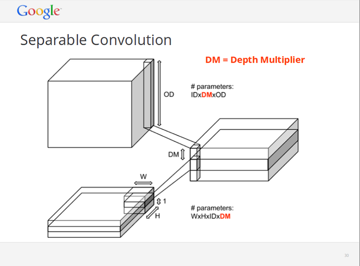
Before diving into this method, be aware that it’s extremely dependent upon how the Separable Convolutions where implemented in a given framework. As far as I am concerned, TensorFlow might have some specific optimizations for this method while for other backends, like Caffe, CNTK or PyTorch it is unclear.

Vincent Vanhoucke, April 2014, “Learning Visual Representations at Scale”
The idea is that instead of convolving jointly across all channels of an image, you run a separate 2D convolution on each channel with a depth of channel_multiplier. The in_channels * channel_multiplier intermediate channels get concatenated together, and mapped to out_channels using a 1x1 convolution.[5] This way one ends up with significantly fewer parameters to train.[2]
# in Keras
from tf.keras.layers import SeparableConv2D
...
net = SeparableConv2D(32, (3, 3))(net)
...
# it's almost 1:1 similar to the simple Keras Conv2D layer
It’s not so simple tho. Beware that Separable Convolutions sometimes aren’t training. In such cases, modify the depth multiplier from 1 to 4 or 8. Also note that these are not that efficient on small datasets, like CIFAR 10, moreover on MNIST. Another thing to keep in mind, don’t use Separable Convolutions in early stages of the network.

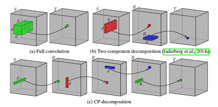
Source: V. Lebedev et al, Speeding-up Convolutional Neural Networks Using Fine-tuned CP-Decomposition
CP-Decomposition and Advanced Methods
The factorization scheme showed above work well in practice, but are quite simple. They work but are by far not the limit of what’s possible. There are numerous works, including [3] by V. Lebedev et al. that show us different tensor decomposition schemes that drastically decrease the number of parameters, hence the number of required computations.
Inspired by [1] here’s a code snippet of how to do CP-Decomposition in Keras:
# **kwargs - anything valid for Keras layers,
# like regularization, or activation function
# Though, add at your own risk

# Take a look into how ExpandDimension and SqueezeDimension
# are implemented in the associated Colab Notebook
# at the end of the article

first = Conv2D(rank, kernel_size=(1, 1), **kwargs)(inp)
expanded = ExpandDimension(axis=1)(first)
mid1  = Conv3D(rank, kernel_size=(d, 1, 1), **kwargs)(exapanded)
mid2  = Conv3D(rank, kernel_size=(1, d, 1), **kwargs)(mid1)
squeezed = SqueezeDimension(axis=1)(mid2)
last  = Conv2D(out,  kernel_size=(1, 1), **kwargs)(squeezed)
It doesn’t work, regretfully, but it gives you the intuition of how it should look like in code. Btw, the image at the top of the article is the graphical explanation of how CP-Decomposition works.
Should be noted such schemes as TensorTrain decomposition and Tucker. For PyTorch and NumPy there’s a great library called Tensorly that does all the low-level implementation for you. In TensorFlow there’s nothing close to it, still, there is an implementation of TensorTrain aka TT scheme, here.
Epilogue
The full code is currently available as a Colaboratory notebook with a Tesla K80 GPU accelerator. Make yourself a copy and have fun tinkering around with the code.
If you’re reading this, I’d like to thank you and hope all of the above written will be of great help for you, as it was for me.
If you are interested in more ML tricks, maybe for other data modalities, be sure to check out the K-Means tricks for fun and profit post.
Let me know what are your thoughs about it in the comments section. Your feedback is valuable for me.
References
- [1] https://medium.com/@krishnatejakrothapalli/hi-rain-4e76039423e2
- [2] F. Chollet, Xception: Deep Learning with Depthwise Separable Convolutions, https://arxiv.org/abs/1610.02357v2
- [3] V. Lebedev et al, Speeding-up Convolutional Neural Networks Using Fine-tuned CP-Decomposition, https://arxiv.org/abs/1412.6553
- [4] C. Szegedy et al, Rethinking the Inception Architecture for Computer Vision, https://arxiv.org/pdf/1512.00567v1.pdf
- [5] https://stackoverflow.com/questions/37092037/tensorflow-what-does-tf-nn-separable-conv2d-do#37092986
- [6] S. Zagoruyko and N. Komodakis, Wide Residual Networks, https://arxiv.org/pdf/1605.07146v1.pdf