MLOps for independent research
19 min read… Or how to run experiments on a budget.
On December 5th, I was presenting online at the Belgium MLOps meetup in Ghent. I thought more people would benefit from the content of that presentation and my experience in general. So, I decided also to have it as an article on my blog. Also, while working on that presentation, I found a few unexpected things, but later about it.
Oh, by the way, one of the best alternative titles was:

Prologue - Some context
I believe it’s important to outline my main research driver:
I’m searching for methods to train strong neural networks from scratch with minimum annotated data. Ideally, with minimum data.
Why? Throughout my career, I had cases when data was scarce and expensive to acquire, and even a pre-trained model couldn’t help. So I had to create small bespoke models to tackle my problems. It was a huge pain, and I want to never go through that hell again and wish no one else would have to either.
Besides, sometimes, using a pre-trained model can be restrictive, depending on its license. Currently, the most relevant type of restrictive license for AI is RAIL. If you wonder why such licenses are restrictive and don’t want to dive into the legal aspects, here are a few good links.
- Evaluating the RAIL license family
- A Reddit discussion about various RAIL variants and their implications
- The New AI Model Licenses have a Legal Loophole | Yannic Kilcher
To form a more nuanced view of ML and licensing, see the two-part essay by Christopher Moran on The Gradient. We won’t dive any deeper in this rabbit hole, otherwise we’ll stray waaaaay too far from this blog’s scope.
So anyway, in the summer of 2021, I had a research internship at Université Paris Sorbonne Nord. I had my own research agenda, and my supervisor was super cool about it. My research project was about searching for more sample-efficient self-supervised learning techniques (SSL). I was working with images, but the method should be modality-agnostic.
The only downside, stemming from my not wanting to work on some existing, grant-covered project, was that I had no access to the necessary hardware.
But that’s alright. It is, isn’t it?
You want to do some independent research
How do you proceed?
Solution: You buy a GPU.
🪄🪄 Or better yet, you buy many GPUs. 🪄🪄
Problem solved.
Bye.
Hold on, seriously. How do you proceed? A good GPU machine will set you back a few thousand USD, even with the crypto boom somewhat behind.
Besides, my project was pretty short-term, so such an investment would be a net loss. And I’m not even counting the time I could spend on it playing games instead of training nets.
And if that wasn’t enough, depending on where you live and the quality of your electric wiring, such a machine will bring more pain and expenses than joy. Have you ever had your personal computer/workstation randomly shutdown due to excesive power consumption, maybe even taking down all your desk appliances with it too? I have.
Free solution: Google Colab
A popular alternative would be to use Google Colab. But not so fast. There are some limitations worth mentioning. Colab’s free tier will only allow you one GPU per account, you have to be mindful of the daily GPU quota (about 8 hours within 24h), and you can’t even run the same notebook in parallel even if it uses the CPU runtime.
What about Colab Pro/Pro+?
- You are not guaranteed any specific GPU. It could be a P100, a T4, or, once in a blue moon, a V100.
- It’s still a single notebook. What if I want multiple?
- What are “compute units”, and how much each GPU costs?
If I am to pay for a service, I’d like to understand what I am paying for and how I’m billed. The opacity of Colab Pro and Pro+ is something I’m not sure I’d be willing to accept.
The first (not so) good solution
Given all that, I decided for my first variant to rely on Colab because it has free access to some GPU resources. With the saved money, I indulged myself with over 20 different kinds of cheese and too many macaron flavors to count. Vive le France!
To run more experiments and somehow circumvent the limited access to GPUs, I was using multiple Google accounts. Each account had a copy of the same Colab notebook and only had to change hyperparameters. If you wonder whether managing these identical-but-not-quite notebooks was a mess, I’ll answer you - it was an absolute mess.
As for my storage solution - I was storing model checkpoints in a shared Google Drive, and given that a blob’s storage consumption is associated with the account that created it and not where it’s stored, in practice, the amount of available Google Drive storage is doubled.
What about experiment tracking? - Google Sheets. Yes, it started to become a mess after the 3rd change of the experiment setup.
Towards a better solution
Of course, it was unsustainable and slow. And painful. And annoying. And somewhat challenging to replicate. So, I needed another solution, and by this time had outlined some constraints:
- Constraint One: Messy environment, mainly Jupyter, with relatively limited code refactoring
- Constraint Two: Ideally, I wanted numerically replicable experiments
- Constraint Three: Also, experiments take a long time, so I want to run many at the same time
- Constraint Four: Cost is a big issue because the research is self-funded
Based on these constraints, I had my core requirements: Cost-efficiency, Flexibility, and Reproducibility. I had some ideas in mind to accomplish these requirements, but I needed computing resources, so my next stop was to use a public cloud.
I picked GCP because I’m most familiar with it. I know about alternative GPU clouds like Paperspace or Linode, but I felt that they might be more expensive. Plus, again, I am most familiar with GCP.

Initially, I was provisioning stuff from the Web console. But it was tedious and error-prone, I like CLIs better, and I had Terraform and Ansible on my radar for a while.
Core requirements: Cost-efficiency
Based on this requirement, here are some decisions that stemmed from it.
- I needed the cheapest powerful machines - Preemptible VMs with GPUs
- I also needed a simple way to quickly spin machines up and down so that I don’t forget anything running and I don’t waste time while setting up the environment - Terraform FTW, and Ansible too
- I had a hunch that by using the most powerful machine and maximizing its usage, I would have the best price-performance ratio - thus, I chose A100 GPUs. To be absolutely honest, another driver for this decision was the coolness factor
- I was running multiple experiments in parallel, as fast as possible - used Papermill for the hands-off launch of multiple notebook-based experiments. Occasionally was using tmux from the Jupyterlab terminal window, but it was a total pain.
- Best cost-optimization is not to run things at all - so I used HPO to select what configurations to run. For HPO, I used Optuna.
Of all the HPO tools out there, why did I choose Optuna, you may ask?
- I like their API. It integrates nicely with Python control structures, like for-loops, or if-elif-else.
- Optuna uses a Bayesian HPO approach. Bayesian methods are pretty accurate and more hands-off than random search, allowing me to launch the hyperparameter search sweep and not think about narrowing down the search space.
- A downside of Bayesian Optimization methods is that they are slow-ish / not very parallelizable. But that’s ok, my degree of parallelization is 2-5 parallel runs, and I didn’t intend to go multi-node.
These decisions converged in the following architecture.
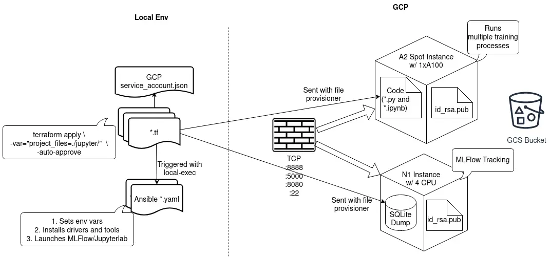
So, a lot of stuff going on here. Let me explain. On the left side, you’ll see the configuration files on the local machine, which are used to instantiate the infrastructure on the right side. Basically, it starts with terraform apply, which reads and executes all terraform files in the project, like this snippet below.
terraform {
  required_providers {
    google = {
      source  = "hashicorp/google"
      version = "3.5.0"
    }
  }
}

provider "google" {
  credentials = file("project-name-some-id.json")

  project = "project-name"
  region  = "${var.region}"
  zone    = "${var.region}-a"
}


resource "google_compute_instance" "vm_instance_worker" {
  name         = "gcp-vm-instance-worker"
  machine_type = "a2-highgpu-1g"

  boot_disk {
    initialize_params {
      image = "deeplearning-platform-release/pytorch-latest-cu110"
      type  = "pd-ssd"
      size  = 150
    }
  }

  metadata = {
    ssh-keys              = "username:${file("~/.ssh/sshkey.pub")}"
    install-nvidia-driver = true
    proxy-mode            = "project_editors"
  }

  scheduling {
    automatic_restart   = false
    on_host_maintenance = "TERMINATE"
    preemptible         = true
  }
}

resource "null_resource" "provision_worker" {
  provisioner "local-exec" {
    command = <<EOF
                ANSIBLE_HOST_KEY_CHECKING=False ansible-playbook \
                -u username \
                -i "${google_compute_instance.vm_instance_worker.network_interface.0.access_config.0.nat_ip}," \
                --extra-vars "tracker_uri=${google_compute_instance.vm_instance_tracker.network_interface.0.access_config.0.nat_ip}" \
                ./config-compute.yml
            EOF
  }
}
The .tf files use the GCP provisioner, and as such, they need a service account key (credentials in provider "google") to be able to provision resources like VMs, buckets, and networks.
Once the infrastructure provisioning part is done, the local-exec provisioner is triggered, which is responsible for running the Ansible playbook and configuring each provisioned VM. It installs drivers, sets env vars, and launches MLFlow or Jupyterlab as background processes. See an example Ansible playbook below.
---
- hosts: all
  name: jupyter-install
  become: username

  tasks:
    - name: install nvidia drivers
      shell: sudo /opt/deeplearning/install-driver.sh

    - name: test nvidia drivers
      shell: /opt/conda/bin/python -c 'import torch; print(torch.cuda.is_available())'
      register: nvidia_test

    - debug: msg="{{ nvidia_test.stdout }}"

    - name: install mlflow
      shell: /opt/conda/bin/pip install mlflow==1.20.2 google-cloud-storage==1.42.3 optuna==2.10.0 papermill==2.3.3

    - name: launch jupyterlab
      environment:
        MLFLOW_TRACKING_URI: 'http://{{ tracker_uri }}:5000'
        MLFLOW_S3_ENDPOINT_URL: gs://some_bucket_address
        PATH: /opt/conda/bin:{{ ansible_env.PATH}}
      shell: "nohup /opt/conda/bin/jupyter lab --NotebookApp.token=some_token --ip 0.0.0.0 --no-browser &"
I am provisioning two VMs, one for the experiment tracker and one for running experiments. I also need a firewall to allow TCP traffic on select ports, specifically 5000 (MLFlow), 8888 (JupyterLab), and 22 (SSH). Finally, I have a GCS bucket as the artifact repository for MLFlow.
Notice that my VMs receive a copy of my SSH public key. It’s necessary to allow SSH connections from my local machine because Ansible uses SSH to connect to its targets.
Core requirements: Flexibility and Parallelism
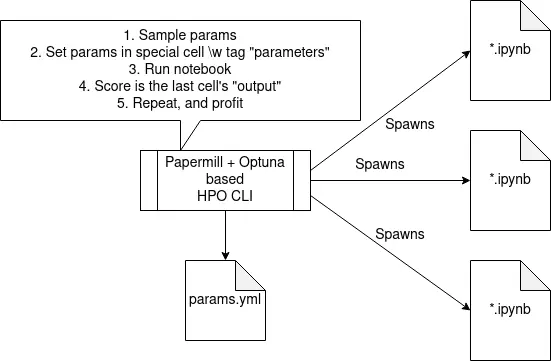
Research is quite messy. I try to fix the mess by extracting common code, maybe writing some utils, but sometimes I prioritize running experiments. As mentioned, I was using Jupyter and Optuna. To make them work nicely together, I used Papermill.
Papermill allows for parametrized, programmatic execution of Jupyter notebooks. Let me explain with a table:
| Capability | Example Usage |
|---|---|
| Parametrizes notebooks | Propose hyperparameters |
| Can inspect them | Extract final scores |
| Executes them | Run notebooks from the command line |
| Stores them | Save specific notebook variants |
So, in my setup a Python CLI program with Optuna and Papermill is used to launch multiple parallel experiments, something like this:
python notebook_hpo.py \
  -i Test.ipynb \
  -o './out/Test.{run_id}.ipynb' \
  -p ./parameters.yml \
  -j 8
Or, if you prefer a diagram to a code snippet, here’s one:
Core requirements: Reproducibility
I have suffered enough in the industry from unreplicable training runs, so I needed to eliminate this issue in my research.
I needed tracking and determinism.
I won’t dive deep into the matter of running reproducible experiments. But I’ll allow myself to repeat some stuff. You can find a more detailed overview here, in the The takeaways > Replicable experiments part.
The deterministic experiments checklist (for PyTorch):
- The most important thing you can do is to seed your pseudo-random number generators (Python, Numpy, PyTorch, CUDA), aka PRNGs.
- Be reasonable about (non-)determinism: Calling
torch.use_deterministic_algorithms()is a Nope for me because it will throw erros when calling.backward()for some layers. On the other hand, settingtorch.backends.cudnn.{benchmark,deterministic}properties is fine; they won’t throw errors. - Special considerations about parallel data loaders, specifically for PyTorch users, don’t forget to also seed them in each of your
DataLoaderworkers, like this:
def seed_worker(worker_id):
    worker_seed = torch.initial_seed() % 2**32
    np.random.seed(worker_seed)
    random.seed(worker_seed)

g = torch.Generator()
g.manual_seed(0)
dl = DataLoader(train_dataset, batch_size=batch_size, num_workers=num_workers,
                worker_init_fn=seed_worker, generator=g)
That’s kind of it with the determinism part. How should I handle my experiment tracking infra?
- I need a minimal, dedicated, non-preemptible VM (
n1-standard-2works fine) because I don’t want my tracking server preempted without first having a DB backup on my laptop, and implementing a half-decent backup script wasn’t something I wanted to do - The experiment tracking server is a self-hosted MLFlow; I am quite familiar with it
- The tracking database is SQLite. SQLite, being basically a single file, allows me to
scpit to my local machine when done working and load it with Terraformfile-provisioneron startup - All my artifacts are checkpointed to GCS, or rather, I’m using GCS as an artifact repository for MLFlow
My tracking strategy:
- Track all modifiable hyper-parameters
- During fine-tuning, track loss, top-1 and top-5 accuracy on both training and validation splits
- During pre-training, only track loss
- No need to track data because I use standard datasets like CIFAR100 or STL10
- Based on my previous experience, I find it quite annoying working with nested runs, so I don’t use those
- I created a new experiment on qualitative/untracked change (a different dataset, changed pre-processing code, a different SSL pre-training method)
Some of it is also explained in detail in that same article referenced above (here it is, for your convenience), in the The takeaways > Experiment tracking part.
Tracking all this stuff with MLFlow, also allows me to compare runs with parallel coordinate plots, which is the best way to look at your hyperparameter optimization runs, IMO!
By the way, if you’re not familiar with MLFlow, here’s a link.
Was it all worth it?
TL;DR: Yes, let me show you why.
First, let’s assume the following setup: ResNet50, pre-training (PT) + fine-tuning (FT), for 10 epochs, with batch sizes 512 (PT) and 4096 (FT).
Let’s first do some benchmarks.
| GPU type | pre-training time | fine-tuning time | compared to A100 |
|---|---|---|---|
| Colab K80 12GB | 965s | 310s | 5.1x slower |
| T4 16GB | 420s | 122s | 2.2x slower |
| A100 40GB | 166s | 80s | 1 |
Let’s do some simple math with the same setup.
A model takes 7.2GB of VRAM. Except for A100, it uses 8.4GB for the same setup. No idea why.
| GPU Type | Nr. of parallel runs |
|---|---|
| Colab K80 12GB | 1 |
| T4 16GB | 2 |
| V100 16GB | 2 |
| A100 40GB | 4 (5 runs with batch_size 448) |
Let’s do some more math.
GCP billed my A2 instance for 44h. Meaning I was running experiments for almost 44h. Of course, I was launching those experiments manually with my script, and there was some idle time, but it was minimal. Anyway, 44 billed hours on A2. For the same volume of work with a T4 GPU, I’d get billed for…
44h x (5 runs / 2 runs) x 2.2 speedup == 240h w/ T4
… for 240 hours. That is a lot more, even if T4 GPUs are considerably cheaper!
Hold on, 5 parallel runs on A100 are possible when using 448 batch size, not 512. That’s almost a 10% smaller batch size, so the training should take roughly 10% more time in this setting. Well, based on a few experiments, changing the batch size from 512 to 448 results in just 3-5% pre-training slowdown, plus there’s the fine-tuning part, which we don’t alter, so all in all, it’s still going to be roughly 2.2x faster than T4.
Anyway, for that 44h I paid 48 USD.
Before we move forward, let’s make one thing clear: based on the information we have so far, Colab Pro/Pro+ is not worth it, compared with my setup, at least.
Colab Pro+ is 43 EUR/month. It does not guarantee the accelerator type, uses opaque “compute units” payment, and 200+h on T4 will consume those units in no time.
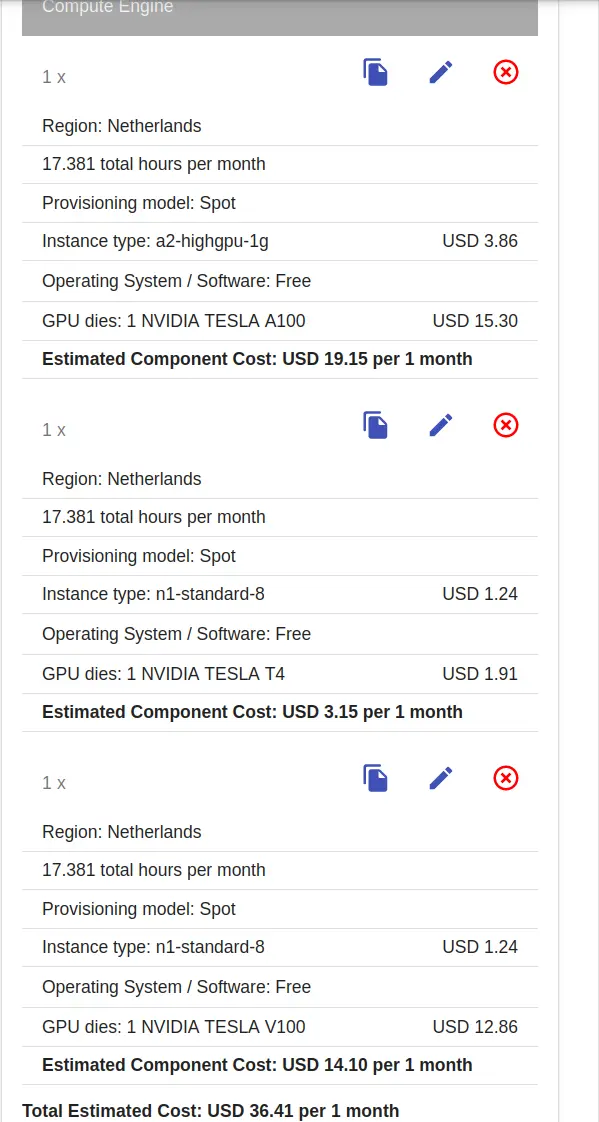
Let’s do some more math. How much would I have to pay for 240h of using a T4 GPU, with a decent VM instance, like an n1-standard-8?
240h x 3.15 USD/h / 17.381h = 43.5 USD
Based on these calculations, I paid a ~5 USD premium for a ~6x speedup. Totally worth it.
In fact, I would have paid more than 43 USD for 240h on T4. Because it seems the network is 1.8-2x slower on N1 instances, resulting in a long time to download the necessary dataset after each provisioning. A few test runs of A2 and N1-standard-8 instances averaged 9m 30s and 19m, respectively, to download the CIFAR100. On a side note, I could have kept copies of the datasets in a GCS bucket, but I didn’t. Maybe I thought it would cost a little too much for its worth, and I’d be annoyed by it. But what’s done is done. Given that I would need to run a T4 instance for considerably longer to do the same amount of work, I’d also have to provision my infrastructure more often, leading to more times I have to wait until my CIFAR100 or STL10 datasets are downloaded. That would definitely result in more than 43 USD.
So A2 is both faster and cheaper in my setup. I wish my gut feeling would always work this well.
So, I hope you can see that using the most expensive single GPU setup on GCP turned out to be the best decision. It costs roughly the same or even less than using the seemingly most cost-efficient one while being soooooo much faster. Even if running an A2 instance was 2x more expensive than N1 with T4 GPU, I’d still take that expense to be able to do 240+h of work in 44h.
Future directions
It may seem like I have my setup optimized to the limit. But it has room for improvement. I’d say the room is the size of a nice large kitchen with an isle in the middle and a terrace for summer dining.
The most impactful missed opportunity is using Mixed Precision. Surprisingly, I wasn’t using it. Maybe because of my old trauma installing APEX from scratch. But now it’s pretty easy, or so they say. Thankfully A100 GPUs have a magic trick, which seems to be enabled by default on PyTorch. This trick is called the TF32 float number representation. It’s a reduced-precision floating point number representation, which can be run on Nvidia’s Tensor Cores and allow for a transparent and easy switch to FP32 when necessary.
A trickier thing I’d like to do is to optimize the data loading. CPUs are underutilized in my setup. Given that my datasets are all standard, I’m considering using FFCV.
A few more niche things, with lower priority than the stuff described above:
- Threaded checkpoint saving because it’s in the same thread as training and takes a few seconds at the end of each epoch.
- Try MosaicML for additional gains. I’m thinking to specifically the ChannelsLast and ProgressiveResizing, but also PyTorch’s OneCycleLR.
- Automatic restart from checkpoints (GCP MIGs + startup scripts) for longer training runs.
Not my case, for now:
- Model/Tensor/Pipeline parallelism - largest model is ResNet101
- Huge datasets - I’m not even planning to use ImageNet
- Collaboration - I was the only one working on it and only discussed the results with my supervisor
A few takeaways
- Automate stuff - I’m sure you’ll be glad you did when you can spin up a complete work setup in minutes with a single click. And shut it down with the same ease. Not to mention leaving an instance running will be a thing of the past.
- Track your experiments - If you want to reproduce your excellent results or figure out what other tricks to try, keeping a log of what you did and how it went is essential.
- Invest in maximizing resource utilization - Having powerful hardware means nothing if it stays idle or is underutilized. Make sure you feed it enough work, so your investment breaks even faster.
- Most powerful hardware can be the most cost-effective - That said, using the newest, most advanced, and most powerful hardware can be not only fun but also cost-effective. And finally,
- Moving faster costs money - but it’s worth it.
P.S.
“Eventually I will buy a GPU”, from the Director of “I will stop binge-playing PS5” and “I promise I’ll go to the gym consistently”.